Devices—How is traffic separation maintained internally to a device? What are the primitives used for Layer 2, Layer 3, or Layer 4 traffic?
Data path—How is traffic separation enforced across a network path? What tools are available to maintain the separation across a network?
Control plane—Because data-path virtualization essentially builds an overlay topology, what changes are needed for routing protocols to function correctly?
This chapter does not cover architectures, topologies, or designs. The purpose of this chapter is to make sure you understand the technology before using it. (The world would be a better place if this principle were universally applied).
The general format for each section of this chapter is to start with a discussion of the protocol technology, highlighting any important details, with some limited configuration examples.
Network Device Virtualization
One of the characteristics of a VN is that it provides what are essentially private communication paths between members of a group over a shared infrastructure. This creates two requirements for the network infrastructure:
Traffic from one group is never mixed with another—For sending and receiving traffic over shared links, tunnels (many borrowed from existing virtual private network [VPN] solutions) can guarantee data separation. Network devices need to enforce group separation in their internal memory (for example, during routing table lookups, access lists processing, or NetFlow statistics gathering).
Each VN has a separate address space—This requirement is derived from the fact that VNs offer the same characteristics as a physical network. Address space and forwarding within it are two of the most basic aspects of any network.
Note – In this section, we start with a narrow definition of device virtualization as creating a separate address space within a network device. However, you can think of this as a special case of a more general definition of a virtualized device, which is the ability for an administrator to allocate device resources to different uses. The first device resource we consider is address space, but as we proceed through both the chapter and book, we include different layers of device policy control mechanisms, such as quality of service (QoS) and security rules. Therefore, the final picture of a virtualized device will be much closer to the general definition.
The first problem to solve is how to virtualize the forwarding plane in a way that meets the requirements for address and traffic flow separation. Depending on the type of device, the virtual separation can go by the following names:
Virtual LAN (VLAN)
Virtual routing and forwarding (VRF)
Virtual forwarding instance (VFI)
Virtual firewall context
Layer 2: VLANs
VLANs are a good example of a piece of the virtualization puzzle that has been around for quite some time. A VLAN is a logical grouping of ports on a switch that form a single broadcast domain. Ports in a VLAN can communicate only with other ports in the same VLAN. How a given switch does this is implementation dependent, but a common solution is for the switch to tag each frame with a VLAN number as it arrives on a port. When a frame is sent to other ports, the output hardware copies the packet only if it is configured with the VLAN number carried in the frame.
On an Ethernet switch, there is typically a single MAC table, which maps ports to MAC addresses. To support VLANs (and simple Layer 2 virtualization), the MAC table has a field for the VLAN number on which the station was discovered, as demonstrated in Example 4-1.
Example 4-1 Switch MAC Table
Switch# show mac-address-table
...
Non-static Address Table:
Destination Address Address Type VLAN Destination Port
------------------- ------------ ---- --------------------
0010.0de0.e289      Dynamic         1 FastEthernet0/1
0010.7b00.1540      Dynamic         2 FastEthernet0/5
0010.7b00.1545      Dynamic         2 FastEthernet0/5
0060.5cf4.0076      Dynamic         1 FastEthernet0/1
0060.5cf4.0077      Dynamic         1 FastEthernet0/1
0060.5cf4.1315      Dynamic         1 FastEthernet0/1
0060.70cb.f301      Dynamic         1 FastEthernet0/1
00e0.1e42.9978      Dynamic         1 FastEthernet0/1
00e0.1e9f.3900      Dynamic         1 FastEthernet0/1
Note – Note that the output in Example 4-1 was taken from https://www.cisco.com/en/US/products/sw/iosswrel/ps5207/products_command_reference_chapter09186a0080417db7.html#wp1021274.
The summary effect of the VLANs is to partition the switch into logical Layer 2 domains. Each domain has its own address space and packets from one domain are kept separate from those of another.
Layer 3: VRF Instances
VRFs are to Layer 3 as VLANs are to Layer 2 and delimit the domain of an IP network within a router. The Cisco website has a more formal definition:
VRF—A VPN Routing/Forwarding instance. A VRF consists of an IP routing table, a derived forwarding table, a set of interfaces that use the forwarding table, and a set of rules and routing protocols that determine what goes into the forwarding table.
Unlike the VLAN scenario, where an extra column in the MAC table is adequate, a VRF partitions a router by creating multiple routing tables and multiple forwarding instances. Dedicated interfaces are bound to each VRF.
Figure 4-1 shows a simple logical representation of a router with two VRFs: RED and GREEN. The RED table can forward packets between interfaces E1/0, E1/2, and S2/0.102. The GREEN table, on the other hand, forwards between interfaces E4/2, S2/0.103, and S2/1.103. An interface cannot be in multiple VRFs at the same time.

Multiple VRFs on a Router
You can see in Figure 4-1 how a VRFs provide separate layer paths between routed interfaces. RED packets can never end up on a GREEN interface.
Note – There is a way to share routes between VRFs, but that is beyond the scope of this introduction. Interested readers should consult the references in the appendix for specialized texts on Multiprotocol Label Switching VPNs (MPLS VPNs).
It is easy to see VRFs on a router. Example 4-2 shows the RED and GREEN VRFs, with their interfaces. Example 4-2 shows overlapping IP addresses on the Serial interfaces. Example 4-3 gives an interface-centric view of the same data.
Example 4-2 Displaying VRFs
Router# show ip vrf
 Name        Default RD     Interfaces
 RED         100:1          Ethernet1/0, Ethernet1/2, Serial2/0.102
 GREEN       100:2          Serial2/0.103, Serial2/1.103, Ethernet4/2
Example 4-3 Displaying interface to VRF mapping
Router# show ip vrf interfaces
Interface      IP-Address    VRF            Protocol
Ethernet1/0    130.22.0.33   RED            up
Ethernet1/2    130.77.0.33   RED            up
Serial2/0.102  130.77.0.33   RED            up
Serial2/0.103  130.77.0.33   GREEN          up
Serial2/1.102  130.77.0.33   GREEN          up
Ethernet4/2    130.22.0.33   GREEN          up
router#
FIBs and RIBs
Before looking at the routing information for a VRF, we need to introduce the routing table’s two main data structures, which are used to find the egress interface for a given packet: the Forwarding Information Base (FIB) and the Routing Information Base (RIB). Long gone are the days when a router maintained a single routing table on which it did linear, longest-prefix searches against destination IP addresses.
The FIB is a database of information used to forward packets. When a packet is received on a routed interface, the router looks up the destination address in the FIB to find the next hop for the packet.
The FIB structure is particularly efficient for resolving longest-prefix matches, and Cisco IOS resolves all route redirections so that a single lookup can yield the entry for the next hop of a packet. Cisco literature often mentions an adjacency concept when presenting the FIB. An adjacency is any node in the network that is reachable with a single Layer 2 hop. It so happens that Cisco IOS also maintains a data structure of adjacencies, which contains, among other things, interface and MAC layer rewrite information for all possible next hops. FIB entries point to the adjacency table, and in the remainder of this chapter, we group the two together and refer simply to the FIB. Hardware-based forwarding paths use the FIB concept, as does Cisco Express Forwarding (CEF).
Because it contains both Layer 2 and Layer 3 information, the FIB can be updated by several sources, such as routing protocol and Address Resolution Protocol (ARP) updates.
The RIB is the memory structure that contains classic routing data. The RIB can contain recursive routes. If a packet destination is not in the FIB, the router “punts” the packet to a slow processing path and resolves the destination next hop using the RIB.
When you enable VRFs, there are multiple instances of information in the FIB and RIB. You can see routing information with show ip route vrf name command, as shown in Example 4-3. Except for the first line, which identifies the VRF, there is no difference from the regular show ip route output.
Example 4-3 VRF Routing Table Information
R104#show ip route vrf RED
Routing Table: RED
Codes: C - connected, S - static, R - RIP, M - mobile, B - BGP
       D - EIGRP, EX - EIGRP external, O - OSPF, IA - OSPF inter area
       N1 - OSPF NSSA external type 1, N2 - OSPF NSSA external type 2
       E1 - OSPF external type 1, E2 - OSPF external type 2
       i - IS-IS, su - IS-IS summary, L1 - IS-IS level-1, L2 - IS-IS level-2
       ia - IS-IS inter area, * - candidate default, U - per-user static route
       o - ODR, P - periodic downloaded static route
Gateway of last resort is not set
   20.0.0.0/24 is subnetted, 1 subnets
O    20.0.0.0 [110/11121] via 40.0.0.1, 00:00:02, Tunnel0
   40.0.0.0/24 is subnetted, 1 subnets
C    40.0.0.0 is directly connected, Tunnel0
   30.0.0.0/24 is subnetted, 1 subnets
C    30.0.0.0 is directly connected, Ethernet0/0
The adjacencies for any routing entry in the VRF must resolve to different interfaces, even if the IP addresses on the interface are identical. Example 4-4 has a FIB entry for 40.0.0.2 from the global routing table, and Example 4-5 has the same information for the RED VRF. These examples are deliberately simple, but you can use the show ip cef forwarding vrf name detail command to peruse the FIB in all its glory.
Example 4-4 FIB Output for Global Routing Table
R104#show ip cef
Prefix          Next Hop       Interface
0.0.0.0/0       drop           Null0 (default route handler entry)
0.0.0.0/32      receive
40.0.0.0/24     attached       Loopback1
40.0.0.0/32     receive
40.0.0.2/32     receive
40.0.0.255/32   receive
Example 4-5 FIB Output for VRF RED
R104#show ip cef vrf RED
Prefix          Next Hop       Interface
0.0.0.0/0       drop           Null0 (default route handler entry)
0.0.0.0/32      receive
40.0.0.0/24     attached       Tunnel0
40.0.0.0/32     receive
40.0.0.2/32     receive
The term global is used to refer to the routing instances and tables that are not in a VRF, as in “global routing table” or “global address space.”
When discussing VRFs, it is common to hear questions about resource allocation, such as “how are router resources allocated between VRFs?” This is a natural question, even if it is not logical! There are no special rules to prioritize data from one VRF to be processed quicker than data from other VRFs. A VRF exists in the memory plane of a device, not in the scheduling plane, which is what per-VRF traffic prioritization would require.
Note – Creating a VRF does not automatically consume a significant amount of memory. However, the expectation is that you will add routes to the VRFs and in this case be careful that the sum of entries in the virtual routing tables does not exceed the capacity of the device. In truth, this is not much different from standard best practices governing route table size.
Traffic processing happens according to the same rules as on a device with no VRFs:
Traffic enters the router.
The ingress policy is applied.
Routing and forwarding lookup occurs.
The egress policy is applied.
Traffic is forwarded.
Obviously, the ingress and egress policies can include QoS statements that prioritize traffic to or from a particular interface or address, but the fact that a packet belongs to a particular VRF has no impact on those policies. It simply alters what happens in Step 3 of the preceding list.
It is far more common to want to bind an interface or packet flow to a particular VRF based on policy criteria. For example, all interfaces from a certain user domain are bound to a single company VRF, or packets with a 10.0.0.0/8 source address are bound to a guest VRF. We look at this in great detail in some of the design chapters.
Virtual and Logical Routers
A VRF is not the same thing as a completely virtualized device, even if they are sometimes confused as such (it is true that some marketing literature encourages such confusion). They simply allow routers to support multiple address spaces. This is some distance from a fully virtualized device, where resources can be more or less arbitrarily allocated to tasks.
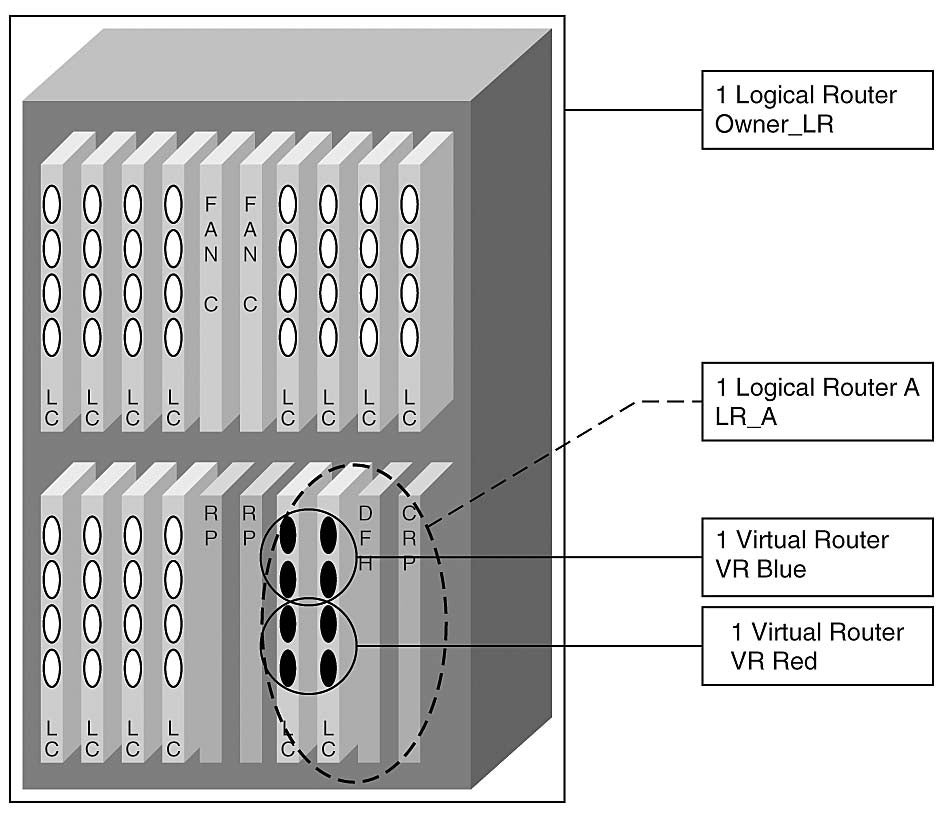
Virtualized devices do exist, however, and, to cut through the fog of confusion, it is helpful to have a taxonomy of terms to start with:
A logical router (LR) uses hardware partitioning to create multiple routing entities on a single device. An LR can run across different processors on different cards of a router. All the underlying hardware and software resources are dedicated to an LR. This includes network processors, interfaces, and routing and forwarding tables. LRs provide excellent fault isolation but do require abundant hardware to implement.
A virtual router (VR) uses software emulation to create multiple routing entities. The underlying hardware is shared between different router processes (note that we mean an entire instance of something like the nonkernel parts of IOS, not a single router process). In a well-implemented virtual router, users can see and change only the configuration and statistics for “their” router.
Note – The previous definitions and Figure 4-2 were derived from RST-4314 2004 Networkers “Advances in Router Architecture: The CRS-1 and IOS-XR,” by David Tsiang and David Ward.
From the preceding list and Figure 4-2, which gives a pictorial idea of the difference between VRs and LRs, you can see that only the LR is completely virtualized. Because of the cost involved of having all that extra hardware and device management, LRs tend to be high-end systems. A VR is a software-based virtualization solution, where all the tasks share the same hardware resources.
In both cases, the granularity of what is virtualized can differ. Some implementations allow multiple router processes (for instance, one VR per customer domain), others allow you to allocate resources to tasks (an LR can have Border Gateway Protocol [BGP] running on one hardware subsystem and Intermediate System-to-Intermediate System [IS-IS] on another, for example).
VRF Awareness
Now that there are multiple routing and forwarding instances on a router, many of the router subsystems that use the information in these tables (which is a long list) need to become “VRF aware.” A VRF-aware feature can be configured to refer to routing and forwarding information from a specific VRF and understand that only certain subinterfaces can be used with certain VRFs. Without this information, the feature uses the global table. For example, to assign an interface to a VRF, the basic interface ip address command was modified to take a VRF name parameter and become ip address vrf NAME forwarding.
Note – VRF awareness is an important implementation detail. Unfortunately, no canonical list exists of VRF-aware features (the list keeps growing), so the best approach is to check the latest online documentation or pester your Cisco representative.
If all features required for a particular application are VRF aware, you can use VRFs to emulate a VR and hence provide virtualized device functionality. This is the approach you will see used in the design sections of this book.
Layer 2 Again: VFIs
VFI is a service-specific partition on a switch that associates attachment circuits in the form of VLANs with virtual switched interfaces (VSIs).
If that did not make much sense, it is useful to have some background on the service itself, namely Virtual Private LAN Services (VPLS), to understand VFIs.
VPLS is a Layer 2 LAN service offered by service providers (SPs) to connect Ethernet devices over a WAN. The customer devices (call them customer edges [CEs] for now; we review this in more detail in Chapter 5, “Infrastructure Segmentation Architectures”) are all Ethernet switches. However, the SP uses a Layer 3 network running Multiprotocol Label Switching (MPLS) to provide this service. The device on the edge of the SP network is called a provider edge (PE). Its role is to map Ethernet traffic from the customer LAN to MPLS tunnels that connect to all the other PEs that are part of the same service instance. The PEs are connected with a full mesh of tunnels and behave as a logical switch, called a VSI. Another way to think about this is to see the VPLS service as a collection of Ethernet ports connected across a WAN. A VSI is a set of ports that forms a single broadcast domain.
In many ways, a VSI behaves just as you would expect a regular switch to. When a PE receives an Ethernet frame from a customer device, it first learns the source address, as would any switch, before looking at the destination MAC address and forwarding the frame. If the port mapping for the destination MAC address is unknown, or is a broadcast, the frame is sent to all PEs that are part of the VSI. The PEs use split horizon to avoid creating loops, which in turn means that no spanning tree is needed across the SP network.
Obviously, the previous explanation hides a fair amount of detail, but it should be enough to give a high-level view of what is going on.
Once again, there is a need to define and manage groups of isolated ports and tunnels on a switch. The VLAN construct is too limited, and a VRF is strictly a Layer 3 affair, so it is necessary to come up with a new virtual device structure for VPLS, called a VFI.
The VFI lists addresses of all the PEs that form a VSI. Recall that VPLS uses a full mesh of point-to-point tunnels for inter-PE connectivity, so there will be connections to each PE listed. The customer-facing ports map VLANs to a VFI name. Example 4-6 shows a short configuration extract that will make this clearer. Figure 4-3 shows the corresponding network topology. The thick line represents the VLAN that runs across the MPLS backbone and connects the VSIs on the PE devices. The CE switches “think” they are connected by a 802.1q trunk on VLAN100. The thin lines between each PE are the actual pseudowires defined in the l2 vfi statement of Example 4-6.
Note – A pseudowire is a tunnel. The term is often used in the context of a Layer 2 service.
VPLS Topology
Example 4-6 VFI Configuration
l2 vfi VPLSA manual
 vpn id 100
 neighbor 13.13.13.13. encapsulation mpls
 neighbor 12.12.12.12 encapsulation mpls

interface loopback 1
 ip address 11.11.11.11 255.255.255.255
interface fastethernet1/0
 switchport
 switchport mode dot1qtunnel
 switchport access vlan 100

interface vlan 100
 no ip address
 xconnect vfi VPLSA
VPLS configuration has two components. The first, which we have already referred to, defines the mesh of pseudowires that together act as a virtual switch. The second maps the VLAN trunk port to a VSI using the xconnect command. This appears at the end of Example 4-6.
Virtual Firewall Contexts
Device virtualization is not limited to switches and routers. As a final example, consider a firewall device. For essentially economic reasons, you might want to share a single firewall between multiple different customers or network segments. Each logical firewall needs to have a complete set of policies, dedicated interfaces for incoming and outgoing traffic, and users authorized to manage the firewall.
Many vendors provide this capability today and undoubtedly have their own, well-chosen name for it, but on Cisco firewalls the term context is used to refer to a virtual firewall. Unlike VRFs, VFIs, or VLANs, a context is an emulation of a device (so an example of the VR concept discussed earlier in this chapter).
Firewall contexts are a little unusual in the way they assign a packet to a context. All the partitions we have seen up to now have static assignment of interfaces (you can assign IP packets to a VRF dynamically. We cover that later). A firewall module looks at an incoming packet’s destination IP address or Ethernet VLAN tag to decide which context a packet belongs to. All the firewall needs is for one of the two fields to be unique. So, either each context has a unique IP address space on its interfaces or the address space is shared, but each context is in a different VLAN.
Figure 4-4 shows a simple setup with an Ethernet switch connected to a firewall context using two VLANs. The switch binds the VLANs to VRF BLUE (at the top) and VRF RED. The firewall has two different contexts. The blue one receives all frames on VLAN 101 and the red one gets VLAN 102. In this way, packets from the outside (on the right side of the figure) that belong to VLAN 101 go through a different set of firewall rules than those belong to VLAN 102.
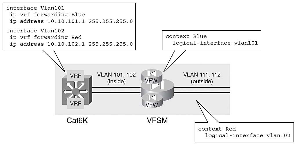
VRF on Switch Connected to Firewall Contexts Across VLANs
Network Device Virtualization Summary
True device virtualization allows resources to be allocated to tasks, or applications. We looked at four different primitives that virtualize the forwarding paths on switches or routers: VLAN and VFI for Layer 2, VRF for Layer 3, and contexts for firewalls. Each of these functions slightly differently. VRFs have the most extensive tie-ins with other features, which we use extensively in the design sections. Before covering data-path virtualization, one word about data center designs. We are focusing on network devices exclusively in this book and do not address the details of server and storage virtualization, which are two important topics in their own right.
Data-Path Virtualization
Connecting devices with private paths over a shared infrastructure is a well-known problem. SPs have solved this with different iterations of VPN solutions over the years. Not surprisingly, we can use and adapt many of these same protocols in enterprise networks to create virtualized Layer 2 and Layer 3 connections using a common switched infrastructure. The focus in this section is on the more relevant of the rather overwhelming menu of protocols to build a VPN. Some of this section is a review for many readers, especially the material on 802.1q, generic routing encapsulation (GRE), and IPsec, and we do not devote much space to these topics. However, we also include label switching (a.k.a. MPLS) and Layer 2 Tunnel Protocol Version 3 (L2TPv3), which are probably less familiar and which consequently are covered in more detail.
Note – In addition to the references listed at the end of the book, we refer interested readers to Appendix A, “L2TPv3 Expanded Coverage,” for more detail about L2TPv3.
Layer 2: 802.1q Trunking
You probably do not think of 802.1q as a data-path virtualization protocol. But, the 802.1q protocol, which inserts a VLAN tag on Ethernet links, has the vital attribute of guaranteeing address space separation on network interfaces.
Obviously, this is a Layer 2 solution, and each hop must be configured separately to allow 802.1q connectivity across a network. Because a VLAN is synonymous with a broadcast domain, end-to-end VLANs are generally avoided.
Generic Routing Encapsulation
GRE provides a method of encapsulating arbitrary packets of one protocol type in packets of another type (the RFC uses the expression X over Y, which is an accurate portrayal of the problem being solved). The data from the top layer is referred to as the payload. The bottom layer is called the delivery protocol. GRE allows private network data to be transported across shared, possibly public infrastructure, usually using point-to-point tunnels.
Although GRE is a generic X over Y solution, it is mostly used to transport IP over IP (a lightly modified version was used in the Microsoft Point-to-Point Tunneling Protocol [PPTP] and, recently, we are seeing GRE used to transport MPLS). GRE is also used to transport legacy protocols, such as Internetwork Packet Exchange (IPX) and AppleTalk, over an IP network and Layer 2 frames.
GRE, defined in RFC 2784, has a simple header, as you can see in Figure 4-5.

GRE Header
The second 2 octets of the header contain the payload protocol type, encoded using Internet Assigned Numbers Authority (IANA) Ethernet numbers (you can find the most recent version on https://www.iana.org/assignments/ethernet-numbers). IP is encoded as 0x800.
The simplest possible expression of a GRE header is a Protocol Type field. All the preceding fields are typically 0, and the subsequent ones can be omitted. You can find freeware implementations that work only with the first 2 octets, but all 4 should be supported.
GRE is purely an encapsulation mechanism. How packets arrive at tunnel endpoints is left entirely up to the user. There is no control protocol, no session state to maintain, no accounting records, and so forth; and this conciseness and simplicity allows GRE to be easily implemented in hardware on high-end systems. The concomitant disadvantage is that GRE endpoints have no knowledge of what is happening at the other end of the tunnel, or even whether it is reachable.
The time-honored mechanism for detecting tunnel reachability problems is to run a dynamic routing protocol across the tunnel. Routing Protocol (RP) keepalives are dropped if the tunnel is down, and the RP itself will declare the neighbor as unreachable and attempt to route around it. You can lose a lot of data waiting for an RP to detect a problem in this way and reconverge. Cisco added a keepalive option to its GRE implementation. This option sends a packet through the tunnel at a configurable period. After a certain number of missed keepalives (the number is configurable), the router declares the tunnel interface as down. A routing protocol would detect the interface down event and react accordingly.
GRE’s lack of control protocol also means that there is essentially no cost to maintaining a quiescent tunnel active. The peers exchange no state information and must simply encapsulate packets as they arrive. Furthermore, like all the data-path virtualization mechanisms we discuss, the core network is oblivious of the number of tunnels traversing it. All the work is done on the edge.
We do not want to suggest that GRE is the VPN equivalent of a universal solvent. There is a cost to processing GRE—encapsulation/decapsulation, route lookup, and so forth—but it’s in the data path.
GRE IOS Configuration
On Cisco devices, GRE endpoints are regular interfaces. This seemingly innocuous statement is replete with meaning, because anything in Cisco IOS that needs to see an interface (routing protocols, access lists, and many more) will work automatically on a GRE tunnel.
Example 4-7 shows a GRE endpoint configuration, corresponding to the R103 router of Figure 4-6.

GRE Topology
Example 4-7 R103 GRE Configuration
interface Tunnel0
 ip address 40.0.0.1 255.255.255.0
 tunnel source Serial1/0
 tunnel destination 192.168.2.1
The tunnel source and tunnel destination addresses are part of the transport network address space. They need to match on both endpoints so that a source address on one router is the destination address on the remote device. The router must also have a path in its routing table to the tunnel destination address. The next hop to the tunnel destination must point to a real interface and not the tunnel interface.
In this case, the router has a tunnel interface with tunnel destination of 192.168.2.1 on the public network. The 40.0.0.0/24 network used for the tunnel IP’s address, however, is part of the private address space used on Sites 1 and 2.
IPsec
IPsec provides a comprehensive suite of security services for IP networks. IPsec was originally conceived to provide secure transport over IP networks. The security services include strong authentication (Authentication Header [AH]) and Encryption (Header [EH]) protocols and ciphers and key-exchange mechanisms. IPsec provides a way for peers to interoperate by negotiating capabilities and keys and security algorithms.
IPsec peers maintain a database of security associations. A security association (SA) is a contract between peers, which defines the following:
The specific encryption and authentication algorithms used, such as Triple DES (Triple Data Encryption Standard)
The IPsec protocol service (Encapsulating Security Payload [ESP] or AH)
Key material needed to communicate with the peer
The SA is negotiated when an IPsec session is initiated. Each IPsec header contains a unique reference to the SA for this packet in a Security Parameter Index (SPI) field, which is 32-bit numeric reference to the SA needed to process the packet. Peers maintain a list of SAs for inbound and outbound processing. The value of the SPI is shared between peers. It is one of the things exchanged during IPsec session negotiation.
At the protocol level, there are two IPsec headers:
AH—Offers nonrepudiatable authentication between two parties. The authentication service also provides for message integrity and certain instances of (identity) spoofing.
ESP—Offers encrypted communication between two parties. The encryption service allows message confidentiality, integrity, nonrepudiation, and protection against spoofing and replay attacks.
It is possible to use authentication and encryption services separately or together. If used in combination, the AH header precedes the ESP header.
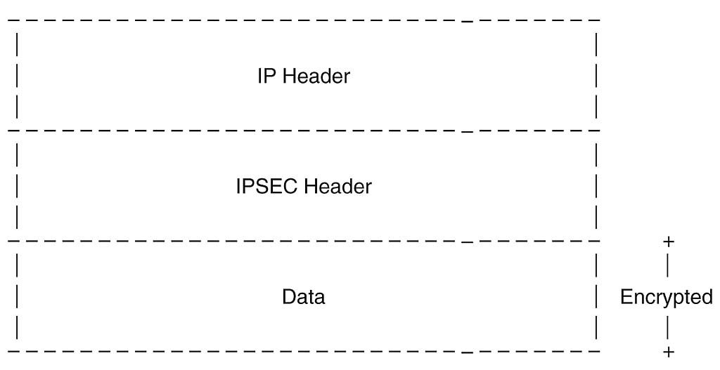
There are two ways to encapsulate IPsec packets. The first, called tunnel mode, encrypts an entire IP packet, including the header, in the IPsec payload. A new IP header is generated for the encrypted packet, as shown in Figure 4-7.

IPsec Tunnel Mode Stack
Tunnel mode adds a 20-octet overload with the new IP header. To reduce issues with packet size and fragmentation, a second mode was defined, called transport mode. Transport mode just protects the TCP/UDP layer and is shown in Figure 4-8. Tunnel mode is better than transport mode at traversing Network Address Translation (NAT) devices.
IPsec Transport Mode Stack
IPsec requires a lot of negotiation to bring up a session. So much so that there is a separate control channel protocol, called Internet Key Exchange (IKE), used to negotiate the SA between peers and exchange keys material. Note that IKE is not mandatory; you can statically configure the SAs.
IKE is not only used during tunnel setup. During confidential data exchange, the session keys used to protect unidirectional traffic may need to be changed regularly, and IKE is used to negotiate new keys.
IKE traffic itself is encrypted, and, in fact, it has its own SA. Most of the parameters are fixed as follows:
56-bit DES for encryption
Message digest 5 (MD5) algorithm or secure hash algorithm (SHA) hashing
Rivest, Shamir, Adleman (RSA) (public key) signatures or preshared keys
IKE runs on UDP/500. IPsec uses IP protocol values of 50 and 51.
Cisco IOS IPsec Configuration
There is a lot more to IPsec than you will see here, but there are three basic parts to the configuration, which correspond to setting up SAs first for IKE, and then for the session itself, and defining which traffic to encrypt. The steps of the configuration are as follows:
The first basic part is the IKE policy. IKE will negotiate its own SA with the remote peer, so it too needs a policy. The crypto isakamp policy command defines the type of authentication, and the IP address of the remote peer and the shared secret used to protect the IKE exchanges, as indicated in Example 4-8.
Example 4-8 IKE Policy Settings
crypto isakmp policy 1
 authentication pre-share
crypto isakmp key secret address 10.0.3.11
In the second basic part is a crypto map, the role of the crypto map is to define the remote peer, the encryption and authentication algorithms (called transforms) that this router will accept to set up a SA, and the interesting traffic to be encrypted. As in so much of Cisco IOS, interesting traffic is defined using standard access lists. If a packet matches an access list entry, whatever IPsec policy is defined in the crypto map is applied to the packet. Example 4-9 has a crypto map that configures any traffic to address 10.0.3.11 that matches access list 101 to be encrypted using the IPsec service called ONE.
Example 4-9 IPsec Crypto Map
crypto map VPN 1 IPsec-isakmp
 set peer 10.0.3.11
 set security-association lifetime seconds 180
 set transform-set ONE
 match address 101
The authentication and encryption algorithms for this SA are defined in a transform set (so they can be shared between multiple SA definitions). The transform set is given in Example 4-10. It specifies AH and ESP services, with MD5 for authentication and DES for encryption.
Example 4-10 IPsec Transform Set
crypto ipsec transform-set ONE ah-md5-hmac esp-des
The third step is to apply the crypto map on an outgoing interface, as in Example 4-11. This completes the puzzle. Now when packets enter or leave the Serial0 interface on this router, they are compared against access list 101 (refer back to the crypto map in Example 4-9), and if there is a match, encrypted according to the service defined in Example 4-10.
Example 4-11 Interface with Crypto Map
interface Serial0
 ip address 10.0.2.11 255.255.255.0
 no ip mroute-cache
 no fair-queue
 crypto map VPN
L2TPv3
Note – Appendix A contains an expanded version of this section that discusses the L2TPv3 protocol in more detail.
The L2TPv3 protocol consists of components to bring up, maintain, and tear down sessions, and the capability to multiplex different Layer 2 streams into a tunnel.
The L2TP protocol has a both a control and data plane. The control channel is reliable. There are 15 different control message types. The major ones are for the setup and teardown of the control channel itself (see Appendix A for more detail). L2TPv3 peers can exchange capability information for the session during the setup phase. The most important of these are the session ID and cookie.
The session ID is analogous to the control channel identifier and it is a “shortcut” value that the receiver associates with the negotiated context for a particular session (for instance, payload type, cookie size, and so forth).
The cookie is an optional, variable-length field of up to 64 bits. The cookie is a cryptographically random number that extends the session identifier space so as to ensure there is little chance that a packet is misdirected because of corrupt session ID. 264 is a large number and, as long as it is random, the cookie makes L2TPv3 impervious to brute-force spoofing attacks, where the attacker tries to inject packets into an active session.
After a session is established through the control session, the L2TP endpoint is ready to send and receive data traffic. Although the data header has a Sequence Number field, the data channel is not reliable. The protocol can detect missing, duplicate, or out-of-order packets, but does not retransmit. That is left to higher-layer protocols.
The RFC allows for the data channel to be set up either using the native control protocol, or statically, or using another control mechanism.
In the design sections after Chapter 5, “Infrastructure Segmentation Architectures: Theory,” you will see occasions when, frankly, GRE could solve a problem just as well as L2TPv3. What then are the differences between these two protocols? Following is a list of them:
Ubiquity—GRE can be found just about everywhere. It is an old (in Internet terms anyway), well-established protocol, and implementations should, by now, be robust. L2TPv3, more recent, is less prevalent.
Performance—On high-speed links, especially on enterprise networks, encapsula-tion tax (header length and so forth) is much less of an issue than a couple of decades ago, when trying to wring every last ounce of baud rate from 1200 bps links was an important issue for network administrators the world over. At Gigabit, or 10 Gigabit speeds, the number of bytes used by a well-designed protocol is not really an issue, as long as the implementation runs in hardware. Concerning this last point, it is probably easier to find hardware implementations of GRE than L2TPv3.
Payload protocols—RFC 3931 specifically states that L2TPv3 is designed to carry Layer 2 protocols. GRE is a multipurpose solution that can carry any other protocol. However, the devil is in the details, and GRE “implementations” may be limited to specific protocols (such as just Ethernet or IP). Furthermore, L2TPv3 has been extended to carry IP traffic.
Cookie—This is the most fundamental difference between the two protocols. GRE has no equivalent of the Cookie field. If this is not important to you—and recall that the main advantage is to provide guarantees against spoofing—implementation issues may dictate your choice more than any difference between the protocols themselves.
L2TPv3 IOS Configuration
There are three things to configure for the L2TPv3 IOS configuration:
Control channel parameters
Data channel parameters
Connection circuit parameters
To configure the first of these parameters, use the l2tp-class command for control channel setup. Here, you can change sequence number settings and so on, but the minimum required is the shared password known to both peers. Example 4-12 demonstrates the use of this command.
Example 4-12 l2tp-class Command
l2tp-class L2WAN
 password 7 00071A150754
As in classic L2TP setup, if you do not give a hostname parameter, the device name is used.
The second part of the configuration is for the data channel. Cisco IOS uses the pseudowire command, which is a generic template also used for Layer 2 over MPLS (called AToM) setup. The pseudowire-class specifies the encapsulation and refers to the control channel setup with the protocol l2tpv3 name command (if you omit this, default control channel settings are used). The pseudowire-class also contains the name of the interface used as the source address of the L2TPv3 packets.
Example 4-13 L2TP pseudowire-class Command
pseudowire-class R103R104
 encapsulation l2tpv3
 protocol l2tpv3 L2WAN
 ip local interface Serial1/0

L2TPv3 Topology
The final part of the configuration (see Example 14-14) binds the client-facing attachment circuit to the trunk port using the xconnect command (already introduced in the discussion on VPLS earlier in this section). The xconnect command defines the remote peer IP address and a unique virtual circuit (VC) identifier used on each peer to map the L2TPv3 payload to the correct attachment circuit. The L2TPv3 endpoints negotiate unique session and cookie ID values for each VC ID, as shown in Figure 4-9. You must configure a different VC ID for each VLAN, port, or data-link connection identifier (DLCI) transported across an L2TPv3 tunnel (currently, Cisco L2TPv3 supports Ethernet, 802.1q [VLAN], Frame Relay, High-Level Data Link Control [HDLC], and PPP).
Example 4-14 xconnect Command
interface Ethernet0/0
 description Client Facing Port
 no ip address
 no cdp enable
 xconnect 192.168.2.1 103 encapsulation l2tpv3 pw-class R103R104
It’s interesting that although the second and third versions of protocol differ in relatively small ways, the command-line interface (CLI) configuration differs significantly from the standard L2TP access concentrator / L2TP network server (LAC/LNS) configuration that you might have used for dialup or digital subscriber line (DSL) networks. However, there are obvious, and deliberate, similarities with other pseudowire solutions such as Ethernet over MPLS (EoMPLS).
Label Switched Paths
Label switched paths (LSPs) are an interesting hybrid of all the preceding data-path solutions: a Layer 2 data path with Layer 3 control plane. Of course, LSPs are found in MPLS networks, which is a topic that has generated entire library shelves of books and other documents. In this chapter, we present a short review of how packets traverse an MPLS network. We do not cover label distribution or any of the major MPLS applications, such as VPN or traffic engineering (MPLS VPNs are discussed in depth in Chapter 5, however).
What we are going to cover may be summarized as follows:
An LSP is a tunnel across an MPLS network made up of individual hop-to-hop segments.
MPLS networks uses the IP control plane.
LSPs are set up for all known IP prefixes in the IP routing table.
LSPs are multiplexed across physical links.
Each node in an MPLS network forwards based on fixed-length labels instead of variable-length prefixes.
Labels are carried in a shim header, between the Layer 2 and Layer 3 headers.
Nodes distribute labels to adjacent nodes using a label distribution protocol.
Basic label switching is easy to configure
Label switching must be configured on all hops.
In a normal routing scenario, when a router needs to forward a packet, it finds the outgoing interface by looking for a matching IP address prefix in the routing table. The actual interface used for forwarding corresponds to the shortest path to the IP destination, as defined by the routing policy. Other administrative policies, such as QoS and security, may affect the choice of interface. This collection of criteria used for forwarding decisions is more generally referred to as a Forward Equivalency Class (FEC). The classification of a packet to FEC is done on each router along the IP path and happens independently of the other routers in the network.
MPLS decouples packet forwarding from the information in the IP header. An MPLS router forwards packets based on fixed-length labels instead of matching on a variable-length IP address prefix. The label is a sort of shortcut for an FEC classification that has already happened. Where the label comes from is discussed later in this section, but for now, it is enough to say that the labels are calculated based on the topology information in the IP routing table. RFC 3031 puts it like this:
In MPLS, the assignment of a particular packet to a particular FEC is done just once, as the packet enters the network. The FEC to which the packet is assigned is encoded as a short fixed length value known as a “label.” When a packet is forwarded to its next hop, the label is sent along with it; that is, the packets are “labeled” before they are forwarded.
In the MPLS forwarding paradigm, once a packet is assigned to a FEC, no further header analysis is done by subsequent routers; all forwarding is driven by the labels.
Before looking at this in more detail, we need to introduce some definitions:
Label switching router (LSR)—A router that switches based on labels. An LSR swaps labels. Unlike a traditional router, an LSR does not have to calculate where to forward a packet based on the IP packet header (which is a simplified way of saying it does not do FEC classification when it receives a packet). An LSR uses the incoming label to find the outgoing interface (and label). LSRs are also called provider (P) routers.
Edge LSR—A router that is on the edge of an MPLS network. The edge LSR adds and removes labels from packets. This process is more formally called imposition and disposition (and also pushing and popping, because labels are said to go on a stack). Edge LSRs are often referred to as provider edge (PE) routers.
Customer edge (CE)—An IP router that connects to the PE device. The CE performs IP forwarding. The PE and CE form routing protocol adjacencies.
Figure 4-10 illustrates MPLS-based forwarding, showing each of the different types of router from the preceding list.

MPLS Forwarding
As a packet flows across the network shown in Figure 4-10, it is processed by each hop as follows:
At the edge of the network, as shown in Figure 4-10, edge LSR A classifies a packet to its FEC and assigns (or imposes) label 17 to the packet. A label is of local significance on that interface just like an ATM VPI/VCI or a Frame Relay DLCI.
In the core, LSRs, such as LSR C and LSR B, swap label values. LSR C removes the old label, 17 in the example shown in Figure 4-10, and imposes the new one, 22. The values of the ingress label and interface are used to find the values of the egress label and interface.
Note – Not all MPLS forwarding modes use incoming interface. Frame mode, used in certain L2VPN services, just uses the incoming label as the same label value is advertised to all peers
LSR B, as the second-last hop in the MPLS network, removes the outermost label from the label stack, which is called penultimate hop popping (PHP). So, packets arrive at edge LSR D without any label, and standard IP routing is used to forward the packet. The process of removing a label is also called disposition. PHP avoids recursive lookups on edge LSR D.
After the label is removed, the packet is forwarded using standard IP routing.
Now the difference with standard IP forwarding should be clearer. FEC classification is done when a packet enters the MPLS network, not at every hop. An LSR needs to look only at the packet’s label to know which outgoing interface to use. There can be different labels on an LSR for the same IP destination. Saying the same thing in a different way, there can be multiple LSPs for the same destination.
A key point to understand is that the control plane is identical in both the IP and MPLS cases. LSRs use IP routing protocols to build routing tables, just as routers do. An LSR then goes the extra step of assigning labels for each destination in the routing table and advertising the label/FEC mapping to adjacent LSRs. ATM switches can also be LSRs. They run IP routing protocols, just as a router LSR does, but label switch cells rather than packets.
What is missing from this description is how label information is propagated around the network. How does LSR A in Figure 4-10 know what label to use? MPLS networks use a variety of signaling protocols to distribute labels:
LDP—Used in all MPLS networks
iBGP—Used for L3 VPN service
RSVP—Used for Traffic Engineering
Directed LDP—Used for L2VPN service, such as VPLS
Label Distribution Protocol (LDP), which runs over tcp/646, is used in all MPLS networks to distribute labels for all prefixes in the nodes routing table. Referring again to Figure 4-10, LSR D and LSR B would bring up a LDP session (LSR B would have another session with LSR C and so forth). LSR D is connected to the customer 192.168.2.0/24 network and advertises this prefix to all its routing peers. LSR D also sends a label to LSR B for the 192.168.2.0 network. When LSR B’s routing protocol converges and it sees 192.168.2.0 as reachable, it sends label 22 to LSR C. This process continues until LSR A receives a label from LSR C.
The complete end-to-end set of labels from LSR A to LSR D form an LSP. An LSP is unidirectional. There is another LSP, identified by a different set of labels, for return traffic from LSR D to LSR A.
Understand that two operations must complete for the LSP from LSR A to 192.168.2.0 to be functional:
The backbone routing protocol must converge so that LSR A has a route to 192.168.2.0.
LDP must converge so that labels are propagated across the network.
Figure 4-10 does not show a numeric value for the label between LSR B and LSR D. In fact, as already discussed, the packet on this link has no label at all, because of PHP. Never-theless, LSR D does still advertise a special value in LDP, called an implicit null (which has a reserved value of 3), so that LSR B performs PHP.
Note – In fact, LSR D might use several special label values for the 192.168.2.0 prefix, such as the aggregate or explicit null.
After LSR A has all the information it needs to forward data across the MPLS network, it encapsulates outgoing packets in a shim header, shown in Figure 4-11 and defined in RFC 3032, which is inserted between the Layer 2 and Layer 3 headers. Encapsulation stacks are defined in different RFCs for Ethernet, ATM, PPP, and other media.
MPLS Shim Header
The MPLS header is simple, as you can see in Figure 4-11. The label itself defines a flat, 20-bit address space. The EXP bits are defined as Experimental, but are in fact used for QoS. MPLS QoS is explained in more detail in the MPLS QoS section of this chapter. The S bit is set on the lowest label when there is more than one label on a packet, which is called a stack. The Time-To-Live (TTL) is analogous to the IP TTL.
Many MPLS applications, such as virtual private networking (VPN) and fast reroute (FRR), involve multiple layers, or stacks, of labels. However, an LSR forwards on the basis of the top, or outer, label values only and never looks at the inner ones.
The FIB Revisited
Label switching adds a forwarding path on a router. The FIB and RIB discussed previously in this chapter contain only IP prefixes. LDP stores labels in a Label Information Base (LIB), and the label values are added to the existing forwarding information in a Label Forwarding Information Base (LFIB). The LDP should have an entry for every non-BGP route in the routing table and all the labels advertised by LDP neighbors. The LFIB is built using a combination of the FIB and LIB. For a given prefix, if there is label in the LIB that is received from the LDP peer address as determined by the FIB, that label is installed in the LFIB and is used for forwarding.
It is important to understand that the LFIB does not replace the FIB. MPLS creates an alternative path through the router. However, IP packets continue to be forwarded using the FIB, and certain special label values can make a router do an FIB lookup.
Cisco IOS LSP Example
Figure 4-12 shows a simple MPLS topology. All routers are running MPLS on their interfaces, with LDP advertising labels to adjacent devices. The core routing protocol is Open Shortest Path First (OSPF), used on all interfaces. The configuration of each device is virtually identical, with the only MPLS-specific commands being activation of LDP (instead of TDP, an earlier alternative) and label switching on each interface, using the mpls ip command (which, for historical reasons, shows up in the output as tag-switching ip). Example 4-15 shows the configuration for R103 in case you want to try this at home.

MPLS Network Topology
Example 4-15 R103 Configuration
mpls label protocol ldp
!
interface Ethernet0/0
 ip address 20.0.0.103 255.255.255.0
 tag-switching ip
!
interface Ethernet1/0
 ip address 192.168.1.1 255.255.255.252
 tag-switching ip
Three show commands enable you to see the mapping of routes from LIB to LFIB. Examples 4-16 through 4-18 give the output of each one in turn and trace labels used to reach R101’s loopback address, 101.101.101.101, from R105. To avoid repetitive output command, we focus on R103 and R102.
Example 4-16 R103 show ip route output
R103#show ip route
Codes: C - connected, S - static, R - RIP, M - mobile, B - BGP
       D - EIGRP, EX - EIGRP external, O - OSPF, IA - OSPF inter area
       N1 - OSPF NSSA external type 1, N2 - OSPF NSSA external type 2
       E1 - OSPF external type 1, E2 - OSPF external type 2
       i - IS-IS, su - IS-IS summary, L1 - IS-IS level-1, L2 - IS-IS level-2
       ia - IS-IS inter area, * - candidate default, U - per-user static route
       o - ODR, P - periodic downloaded static route
Gateway of last resort is not set
   101.0.0.0/32 is subnetted, 1 subnets
O    101.101.101.101 [110/21] via 20.0.0.102, 00:12:25, Ethernet0/0
   20.0.0.0/24 is subnetted, 1 subnets
C    20.0.0.0 is directly connected, Ethernet0/0
   10.0.0.0/24 is subnetted, 1 subnets
O    10.0.0.0 [110/20] via 20.0.0.102, 00:12:25, Ethernet0/0
   192.168.1.0/30 is subnetted, 1 subnets
C    192.168.1.0 is directly connected, Ethernet1/0
   192.168.2.0/30 is subnetted, 1 subnets
O    192.168.2.0 [110/20] via 192.168.1.2, 00:12:25, Ethernet1/0
   30.0.0.0/24 is subnetted, 1 subnets
O    30.0.0.0 [110/30] via 192.168.1.2, 00:12:25, Ethernet1/0
There is a one-to-one mapping between the content of the routing table in Example 4-16 and the LIB of Example 4-17. The LFIB, shown in Example 4-18, only contains labels for LSPs that cross the device. If an MPLS packet arrives with an unknown label, it is dropped.
Example 4-17 R103 Label Information Base
R103#show mpls ldp bindings
 tib entry: 10.0.0.0/24, rev 10
    local binding: tag: 17
    remote binding: tsr: 192.168.1.2:0, tag: 17
    remote binding: tsr: 20.0.0.102:0, tag: imp-null
 tib entry: 20.0.0.0/24, rev 8
    local binding: tag: imp-null
    remote binding: tsr: 192.168.1.2:0, tag: 16
    remote binding: tsr: 20.0.0.102:0, tag: imp-null
 tib entry: 30.0.0.0/24, rev 12
    local binding: tag: 18
    remote binding: tsr: 192.168.1.2:0, tag: 18
    remote binding: tsr: 20.0.0.102:0, tag: 18
 tib entry: 101.101.101.101/32, rev 14
    local binding: tag: 19
    remote binding: tsr: 20.0.0.102:0, tag: 19
    remote binding: tsr: 192.168.1.2:0, tag: 19
 tib entry: 192.168.1.0/30, rev 5
    local binding: tag: imp-null
    remote binding: tsr: 192.168.1.2:0, tag: imp-null
    remote binding: tsr: 20.0.0.102:0, tag: 16
 tib entry: 192.168.2.0/30, rev 6
    local binding: tag: 16
    remote binding: tsr: 192.168.1.2:0, tag: imp-null
    remote binding: tsr: 20.0.0.102:0, tag: 17
Example 4-18 R103 Label Forwarding Information Base
R103#show mpls forwarding-table
Local Outgoing   Prefix         Bytes tag  Outgoing   Next Hop
tag   tag or VC  or Tunnel Id   switched   interface
16    Pop tag    192.168.2.0/30  0         Et1/0      192.168.1.2
17    Pop tag    10.0.0.0/24     0         Et0/0      20.0.0.102
18    18         30.0.0.0/24     0         Et1/0      192.168.1.2
19    19         101.101.101.101/32
                                 0         Et0/0      20.0.0.102
Figure 4-12 shows the label values advertised by each LSR for prefix 101.101.101.101. Example 4-18 shows how this label information appears in R103’s LIB. There are three entries for 101.101.101.101:
local binding—The router’s own, called local, which is advertised to downstream neighbors
20.0.0.102:0, tag: 19—The label advertised by the upstream router R102
192.168.1.2:0, tag: 19—The label advertised by the downstream router SP107
In the LFIB in Example 4-18, there is a single entry for 101.101.101.101/32. It means that R103 will forward a packet received with value 19 onto interface Ethernet0/0. R103 also swaps the label value. It is just a coincidence that the same values are used for the same IP prefix on different routers. Labels have local significance.
Figure 4-12 shows that router R102 receives an implicit null label from R101 and so performs PHP with label value 19 and forwards an IP packet on interface Ethernet0/0.
Data-Path Virtualization Summary
We presented several different protocols that can be used for data-path virtualization. Two of them are suitable for Layer 2 traffic only: 802.1q, which is configured on each hop, and L2TPv3 which is configured end to end. IPsec is suitable for IP transport. Finally, GRE and MPLS LSPs can be used for either Layer 2 or Layer 3. GRE is another IP tunnel protocol, configured only on endpoints. MPLS creates a new forwarding path and is configured on all hops in a network.
Control-Plane Virtualization—Routing Protocols
Data-path virtualization essentially creates multiple separate logical networks over a single, shared physical topology. To move packets across these VNs, you need to need a routing protocol.
The most familiar virtualized control plane is probably Per VLAN Spanning Tree (PVST), which has a separate spanning-tree instance for each VLAN running on a switch. Even through PVST has been around longer than the term virtualization, it illustrates the central point we are making here very crisply. Different logical networks have different topologies and, therefore, different optimal paths. Switches have to run different spanning-tree calculations for each such network.
The remainder of this section deals with extensions to routing protocols to allow them to run with multiple routing instances. However, we will return to the topic of control-plane virtualization, because many different router and switch functions, such as NetFlow, DHCP, RADIUS, and so on, need to receive the same treatment and become VRF aware.
Note – The need for VRF awareness was introduced in the section on device virtualization earlier in the chapter. This is particular to Cisco platforms. In more general terms, features applied or related to the data path, such as NetFlow, RADIUS, and so on, need to support virtualization also—it’s not as simple as creating multiple routing tables.
VRF-Aware Routing
Cisco’s major interior gateway protocol (IGP) routing protocol implementations are VRF aware. This means that they understand that certain routes may be placed only in certain routing tables. The routing protocols manage this by peering within a constrained topology, where a routing protocol instance in a VRF peers with other instances in the same VN. No special information is added to the route advertisements to identify VRF names, so routing instances must communicate over private links.
With some protocols (for example, BGP), a single routing instance can manage multiple VRF tables; with others (for example, OSPF), a different routing process runs for every VRF. Remember that in both cases, every VRF requires a route optimization calculation, so increasing the number of VRFs does have a computational impact on a network device.
Chapter 5 has more information on the end-to-end setup. This section just covers the main concepts.
VRF per Process: OSPF
OSPF has a different routing process for each VRF. The first implementation was rather strict, with a maximum of 32 processes. Furthermore, two processes are reserved for static and connected routes. Recent software enhancements lift this limitation. You are now limited to 32 VRFs per process, but the number of processes is now fixed by the network devices’ CPU and memory limitations (300 to 10,000 depending on the platform).
Example 4-19 shows how an OSPF process is associated with the RED VRF. The networks advertised by this process should be in the same VRF.
Example 4-19 Per-VRF OSPF Configuration
router ospf 2000 vrf RED
 log-adjacency-changes

 network 20.0.0.0 0.0.0.255 area 0
 network 40.0.0.0 0.0.0.255 area 0
VRF Address Families: EIGRP, RIP, and BGP
For the other routing protocols, a single process can manage all the VRFs, and the Cisco IOS address-family command is used to configure per-VRF route policy. Example 4-20 shows how to configure RIP for two VRFs, RED and GREEN. Each VRF has overlapping entries for network 13.0.0.0.
Example 4-20 Per-VRF RIP Configuration
router rip
 version 2
 !
 address-family ipv4 vrf RED
 version 2
 network 11.0.0.0
 network 13.0.0.0
 no auto-summary
 exit-address-family
 !
 address-family ipv4 vrf GREEN
 version 2
 network 12.0.0.0
 network 13.0.0.0
 no auto-summary
 exit-address-family
!
Example 4-21 shows an iBGP per-VRF Configuration.
Example 4-21 Per-VRF iBGP Configuration
router bgp 100
 no synchronization
 bgp log-neighbor-changes
 no auto-summary
 !
 address-family ipv4 vrf RED
 redistribute connected
 neighbor 14.0.0.1 remote-as 100
 neighbor 14.0.0.1 update-source loopback100
 neighbor 14.0.0.1 activate
 no auto-summary
 no synchronization
 exit-address-family
 !
 address-family ipv4 vrf GREEN
 redistribute connected
 neighbor 15.0.0.1 remote-as 100
 neighbor 15.0.0.1 update-source loopback200
 neighbor 15.0.0.1 activate
 no auto-summary
 no synchronization
 exit-address-family
!
Multi-Topology Routing
Multi-Topology Routing (MTR) is a recent innovation at Cisco. As the name suggests, it creates multiple routing topologies across a shared, common infrastructure. However, MTR does not try to be yet another VPN solution. Instead, it creates paths through a network that you can map to different applications or classes of applications, with the understanding that, by separating traffic in this way, you can provide better performance characteristics to certain critical applications.
MTR bases its operation on the creation of separate RIBs and FIBs for each topology. The separate RIBs and FIBs are created within a common address space. Thus, MTR creates smaller topologies that are a subset of the full topology (also known as the base topology). The main difference between MTR and a VPN technology is that, with MTR, a single address space is tailored into many topologies that could overlap; whereas VPNs create totally separate and independent address spaces.
Thus, MTR must carry out two distinct functions:
At the control plane—Color the routing updates, so that the different topology RIBs are populated accordingly. Based on these RIBs, the corresponding FIBs are to be written.
At the forwarding plane—Identify the topology to which each packet belongs and use the correct FIB to forward the packet.
At each hop, there will be a set of prefixes and routes in the RIB for each topology. The contents of these RIBs are dynamically updated by routing protocol colored updates. Based on this RIB information, a separate FIB is built for each topology.
To forward traffic over different topologies, the router looks for a code point in each packet and chooses an FIB based on this code point. A first implementation of MTR uses differentiated services (DiffServ) code point (DSCP) as such a code point, but other code points could be used by future implementations. The DSCP value is used as a pointer to the correct forwarding table, and the packet’s destination address is used to make a forwarding decision based on the information in the topology’s FIB. MTR uses the terminology of color to refer to separate topologies. So, a RED value in a packet’s DSCP field is recognized by the router, which will forward the packet using the RED forwarding table (FIB).
MTR must run contiguously across a network, and the color mappings must be consistent (that is, you cannot use DSCP X as Green on one hop but as Red on the next). MTR does not allow you to double dip: If the destination route is not in the routing table of the color a packet is using, the packet can either be dropped or forwarded over the base topology—there are no lookups in “backup topologies” other than the base topology (which is equivalent to regular routing).
MTR does not change how routing works; it just runs across multiple topologies (using a single process with colored updates).
Control-Plane Virtualization Summary
Control-plane virtualization refers to adaptations made to routing protocols to be able to operate on virtualized devices. We concentrated on per-VRF routing because that is the main tool we use for design. However, VRs and LRs also run separate routing instances in a similar manner to the one shown here. In all cases, there are no changes to the protocol “on the wire.” MTR is an interesting new development that can also be categorized in the virtualized control-plane bucket.
Summary
This chapter covered a lot of ground. The basic idea is that there are different levels of virtualization: device, data path, and control path. There are different constructs and protocols to implement for each of these, and, depending on the problem you need to solve, you can combine these to arrive at an overall network design.
This chapter avoided all discussion of architecture, the better to focus on protocol and implementation details. The next chapter covers hub-and-spoke and RFC 2547 architectures.
Copyright © 2007 Pearson Education. All rights reserved.